Vector Winds
Written on March 19th, 2023 by Brandon Kerns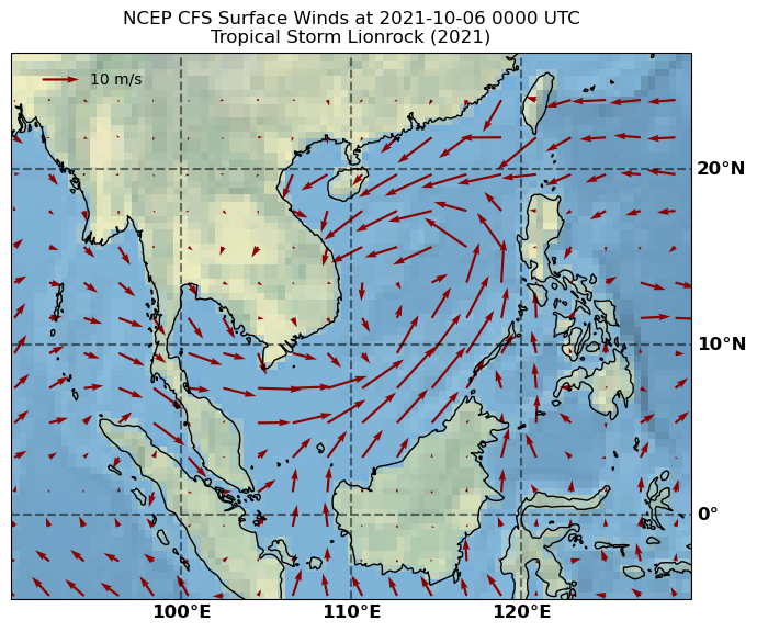
Plot a wind vector map using OpenDAP data.
1. Import modules and specify global settings.
We use a Mercator projection for the map in this case, since it is in the tropics. Details on other projections that can be used with Cartopy are here:
PROJ_latlon is the "source" projection, i.e., the projection that the wind data are provided on. PlateCarree() is Cartopy's fancy term for a regular lat-lon grid.
import numpy as np
import xarray as xr
import datetime as dt
import matplotlib.pyplot as plt
import matplotlib.ticker as mticker
import cartopy
import cartopy.crs as ccrs
# import cartopy.mpl.ticker as cticker
from cartopy.mpl.gridliner import LONGITUDE_FORMATTER, LATITUDE_FORMATTER

plt.close('all')

## Define the map projections that I need.
PROJ = ccrs.Mercator()
PROJ_latlon = ccrs.PlateCarree()
PLOT_AREA = [90, 130, -5, 25]
2. Read in some wind data.
Notes:
- These data come with latitude "reversed"--from NORTH to SOUTH.
- To deal with this, the latitude values in the slice are also "reversed."
- Quiver wants x and y values monotonically increasing. Therefore, flip the Y dimension.
this_time = dt.datetime(2021,10,6,0,0,0) ## 2021-10-06 0000 UTC, Tropical Storm Lionrock (2021)
url='https://rda.ucar.edu/thredds/dodsC/files/g/ds094.1/2021/wnd10m.cdas1.202110.grb2'

with xr.open_dataset(url) as DS:
    DS_this_time = DS.sel(time=this_time, lon=slice(PLOT_AREA[0], PLOT_AREA[1]), lat=slice(PLOT_AREA[3], PLOT_AREA[2]))
    print(DS_this_time)

    X = DS_this_time['lon'].data
    Y = DS_this_time['lat'].data
    U = DS_this_time['u-component_of_wind_height_above_ground'].data[0,:,:]
    V = DS_this_time['v-component_of_wind_height_above_ground'].data[0,:,:]

## Y coordinate in this case is reversed, so flip the Y (lat) direction.
Y = np.flip(Y)
U = np.flipud(U)
V = np.flipud(V)
<xarray.Dataset>
Dimensions:                                  (lat: 146, lon: 195, height_above_ground: 1)
Coordinates:
  * lat                                      (lat) float32 24.84 ... -4.804
  * lon                                      (lon) float32 90.2 90.41 ... 129.9
    time                                     datetime64[ns] 2021-10-06
    reftime                                  datetime64[ns] ...
  * height_above_ground                      (height_above_ground) float32 10.0
Data variables:
    GaussLatLon_Projection                   int32 ...
    u-component_of_wind_height_above_ground  (height_above_ground, lat, lon) float32 ...
    v-component_of_wind_height_above_ground  (height_above_ground, lat, lon) float32 ...
Attributes:
    Originating_or_generating_Center:                                        ...
    Originating_or_generating_Subcenter:                                     ...
    GRIB_table_version:                                                      ...
    Type_of_generating_process:                                              ...
    Analysis_or_forecast_generating_process_identifier_defined_by_originating...
    file_format:                                                             ...
    Conventions:                                                             ...
    history:                                                                 ...
    featureType:                                                             ...
3. Make the map plot.
We first define a function for generating the map background. This avoids some code repetition.
## First define a function for creating the map background.
def set_up_figure(proj, plot_area=[-180, 180, -80, 80]):
    fig = plt.figure(figsize=(8,8))
    ax = fig.add_subplot(1,1,1, projection=proj)
    ax.coastlines()

    ax.set_extent(plot_area)

    return(fig, ax)
3.1. Initial "dummy" version
This draws every point, which is way too much data!
fig, ax = set_up_figure(PROJ, plot_area=PLOT_AREA)
Q = ax.quiver(X, Y, U, V, color='b', transform=PROJ_latlon)
qk = ax.quiverkey(Q, 0.10, 0.95, 10, '10 m/s', labelpos='E', transform=PROJ_latlon)

3.2. Skip vectors, plot every nth wind vector.
In this case, plotting every 10th vector works out good.
# Skip every nth wind vector.
skipx = 10
skipy = 10

fig, ax = set_up_figure(PROJ, plot_area=PLOT_AREA)
Q = ax.quiver(X[::skipx], Y[::skipy], U[::skipy,::skipx], V[::skipy,::skipx], color='b', transform=PROJ_latlon)
qk = ax.quiverkey(Q, 0.10, 0.95, 10, '10 m/s', labelpos='E', transform=PROJ_latlon)

3.3. Control the vector length.
The above looks OK, but usually we want to control the vector length.
I prefer to scale it according to "inches", e.g., 1 inch is 10 m/s.
We can also customize the quiver key.
# Skip every nth wind vector.
skipx = 10
skipy = 10
scale = 30 # m/s for 1 inch.

fig, ax = set_up_figure(PROJ, plot_area=PLOT_AREA)
Q = ax.quiver(X[::skipx], Y[::skipy], U[::skipy,::skipx], V[::skipy,::skipx]
              , color='b', transform=PROJ_latlon
              , scale=scale, units='inches')
qk = ax.quiverkey(Q, 0.10, 0.95, 10, '10 m/s', labelpos='E', transform=PROJ_latlon)

Refine the map background.
We've got the vectors in good shape, but the map background can be improved! Let's define a new map backgroud function that does the following:
- Color shaded map background.
- Add latitude and longitude grid lines and labels.
- Dark red vectors contrast better with the background.
Finally, we add a title and save the output image to vector_wind_map.png.
## First define a function for creating the map background.
def set_up_figure_prettier(proj, plot_area=[-180, 180, -80, 80]):
    fig = plt.figure(figsize=(8,8))
    ax = fig.add_subplot(1,1,1, projection=proj)
    ax.stock_img()
    ax.coastlines()

    ax.set_extent(plot_area)

    ## Set up grid lines and axis labels.
    gl = ax.gridlines(crs=ccrs.PlateCarree(), linewidth=1.5, color='black', alpha=0.5, linestyle='--', draw_labels=True)
    gl.top_labels = False
    gl.left_labels = False
    gl.xlines = True
    gl.xlocator = mticker.FixedLocator([90, 100, 110, 120, 130])
    gl.ylocator = mticker.FixedLocator([0, 10, 20])
    gl.xformatter = LONGITUDE_FORMATTER
    gl.yformatter = LATITUDE_FORMATTER
    gl.xlabel_style = {'color': 'black', 'weight': 'bold', 'fontsize': 12}
    gl.ylabel_style = {'color': 'black', 'weight': 'bold', 'fontsize': 12}

    return(fig, ax)

# Skip every nth wind vector.
skipx = 10
skipy = 10
scale = 30 # m/s for 1 inch.

fig, ax = set_up_figure_prettier(PROJ, plot_area=PLOT_AREA)
Q = ax.quiver(X[::skipx], Y[::skipy], U[::skipy,::skipx], V[::skipy,::skipx]
              , color='darkred', transform=PROJ_latlon
              , scale=scale, units='inches')
qk = ax.quiverkey(Q, 0.10, 0.95, 10, '10 m/s', labelpos='E')

ax.set_title('NCEP CFS Surface Winds at 2021-10-06 0000 UTC\nTropical Storm Lionrock (2021)')

plt.savefig('vector_wind_map.png', dpi=100, bbox_inches='tight', background_color='white')